This is part one of a summary I am writing for the paper "A primer on encoding models in sensory neuroscience" by Marcel A.J. van Gerven. Today's post is on chapter 1.3.
Defining x(t), a(t) and y(t)
Encoding consists of mapping sensory stimuli to neural activity or, more accurately, measurements of neural activity.
The sensory stimuli can be thought of as a vector x. For visual stimuli, each entry could be the intensity of a pixel for example. We call x the input vector. x(t) equals the input vector at time t.
If we separate the brain into p distinct neural populations, we can think of neural activity as a vector a with an entry for the aggregate neural activity in each population. a(t) is the neural activity at time t.
We can't measure neural activity directly, though. Instead, we make measurements from sensors. A sensor could be a voxel in an fMRI scan for example.
If we have q sensors we can put all our measurements into a vector y with q entries. y(t) is our measurements at time t.
Lets redefine our problem
Instead of choosing a specific encoding for our stimuli, we could calculate a probability distribution. A probability distribution is a tool we can use to ask questions like, "Given this sequence of input vectors {x(0), x(1), ...}, what is the probability we will make these measurements {y(0), y(1), ...}?".
In other words, we can describe an encoding model as a mathematical framework for quantifying which measurements are likely depending on the stimuli. Using an encoding model to make predictions about measurements is how neural encoding is implemented in practice.
In order to calculate the probability distribution we need to understand the relationships between x(t), a(t) and y(t).
y depends on a depends on x
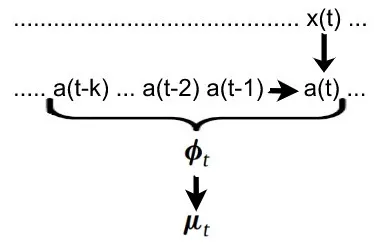
Let's first quantify the relationship between x(t) and a(t). We know that, somehow, a(t) must depend on x(t) because neural activity reacts to outside stimuli. a(t) can then influence future activity when the brain continues processing the information. Another way of saying this is that the current neural activity not only depends on the current stimuli, but also on the previous neural activity.
We can write: a(t) = g(x(t), a(t-1)) where g is some nonlinear function.
We have a similar situation when defining the relationship between a(t) and y(t). Due to lagging and other signal-altering effects, y(t) depends not only on the current neural activity a(t), but on the "history" of neural activity.
For brevity we can call the history (a(t), a(t-1), a(t-2), ... , a(t-k)) the feature space phi(t). Each entry can be calculated with g. (see above)
Since we are dealing with probabilities, we don't calculate the measurements from the neural activity directly. Instead we calculate the expected value.
mu(t) = f(phi(t)) where mu(t) is the expected value of y(t) and f is called the forward model.
You can think of the forward model as a function which calculates the most likely measurement given the feature space. In other words, f maps a history of neural activity to the likeliest resulting measurement.
Conclusion
Now that we understand how to calculate the expected measurement vector mu(t) from the input vector x(t), we need to put everything together to get a probability distribution. That will be the topic of the next post.