Let's take a peek into a more advanced area of study in the field of differential equations. A few days ago 
So I thought we could explore this model a bit further and develop the logic behind it.
Suppose we have a prey species (for example: rabbits) that serves as a food source for a predator species (for example: foxes).

First, let the number of rabbits (i.e. population) be denoted by R.
Now, assuming there are no predators around, and they have indefinite lives, and infinite resources and space in which to thrive, the growth in the population of rabbits can be modeled by natural growth (aka exponential growth), or the equation...

For foxes, assuming they have no food supply (no prey) we would expect their population, denoted by F to naturally decline (aka exponential decay) according to the equation...

Let's now bring predator and prey together so they start encountering or "interacting" with each other. So let the number of encounters be the product of the number of foxes by the number of rabbits.
Obviously this is very simplistic, but what this means is the number of encounters depends on the number of either species. So we define...

Unfortunately, for the prey that means being eaten by the predators. So we would expect their population growth to be slowed in proportion to the number of encounters, expressed as 

For the predators, we would expect the change in their population to be boosted in proportion to the number of encounters since they now have a food source (

Equations (3) and (4) together, are a system of first order differential equations called the "Lotka-Volterra" equations (or simply, predator-prey equations).

They are a pair of non-linear differential equations which must be solved simultaneously, and the solution is likewise, a pair of functions R(t) and F(t).
Now unfortunately, explicit solutions to R(t) and F(t) are usually impossible to find. Most of the time, they are approximated by "linearising" the non-linear system, or using a numerical integrating method. This is too complex for us (i.e. for me, as I'm still revising and learning) at this stage, but we still have plenty to explore...
For the following example, let's set some values...
- k = 0.05
- c = 0.018
- α = 0.002
- β = 0.00002
Equilibrium solutions to the Lotka-Volterra Equations
As always, equilibrium points (or critical points) are where the rate of change in population is equal to zero. To find these, we simply set equation (3) equal to 0...

The above as solutions R = 0 and F = k/α = 0.05/0.002 = 25.
Likewise, we also set equation (4) equal to 0...

Has solutions F = 0 and R = c/β = 0.018/0.0002 = 900.
What this physically means is populations of either species can be sustained indefinitely when...
There are no foxes and rabbits in the ecosystem whatsoever, (R,F) = (0,0). And this sort of makes sense because if neither species existed in the first place, then their populations would not change (unless they may evolve into existence over a very long time ... but that's a controversial debate for another day).
The number of foxes is 25 and the number of rabbits is 900 (R,F) = (900,25). Or in other words, 900 rabbits is just enough to support 25 foxes. There are neither too few foxes such that the population of rabbits increases, nor too many foxes such that their numbers decline.
Phase portrait solution
While we may not easily be able to obtain the functions R(t) and F(t), we can still obtain in my opinion, an even more meaningful relationship between the number of foxes to rabbits with what is known as a phase portrait that is independent of time.
To do this, we use the chain-rule to eliminate time t and find an expression for dF/dR...

The direction field shown in Figure 1 will give us an idea of the solutions we can obtain from equation (6)...
Figure 1.

Equation (6) is a separable differential equation. So, the variables can be separated and then the equation solved by integrating both sides...

Substituting the numerical values, we get the general solution...

Several solution curves of the phase portrait for foxes versus rabbits is shown in Figure 2.
Figure 2.

The egg shaped curves show how the population of either species changes with respect to each other. The equilibrium solution of 900 rabbits to 25 foxes lies at the centre of these curves.
The outer orange curve in Figure 2 is a particular solution where we start at t0 with 900 rabbits and only 10 foxes.
If we follow this curve in the anti-clockwise direction as time progresses, we see that the increase in the number of foxes is very gradual compared to the number of bunnies because there are not enough foxes to significantly slow the increase in their population.
However, because the foxes have plenty of food (prey), their rate of population increase gets faster and faster until there are about 2800 rabbits in the ecosystem, the point at which the population of rabbits begins to decrease, t1. The number of rabbits cannot continue to grow because there are 25 foxes catching them.
The fox population continues to grow as the number of rabbits decreases albeit at a slower rate until they number 50 at t2. After this, both populations are in decline. There are too many foxes and they have consumed so many rabbits that they are exhausting the food supply, and their numbers decline rapidly.
At t3, foxes are still in rapid decline while the rabbit population starts to recover and increase again. As time goes on, the rate of fox depopulation slows as their food supply increases again until we reach a point similar to when we started at t0.
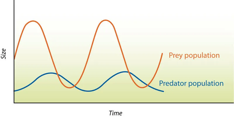
A typical plot of each population over time is shown in Figure 3 below. As you can see, there is a phase lag for the predator population which makes sense according to the description of the phase portrait above.
Figure 3.
Image Source
Assumptions of the standard Predator-Prey model
The example described above is the standard model first described by Lotka & Volterra in the 1920's. Several assumption are made to simplify the model that are not necessarily realisable in nature.
They are:
- The prey population finds ample food at all times.
- The food supply of the predator population depends entirely on the size of the prey population.
- The rate of change of population is proportional to its size.
- During the process, the environment does not change in favour of one species and genetic adaptation is inconsequential.
- Predators have limitless appetite.
Many variations of the Lotka-Volterra equations have been proposed to take into account natural factors (such as the environment, food supply for the prey etc.) that may effect the growth rates of the species in question. We'll leave these for another time.
Credits:
All equations in this tutorial were created with QuickLatex
All graphs were created with www.desmos.com/calculator
Introduction to First Order Differential Equations
First-Order Differential Equations with Separable Variables - Example 1
Exponential Decay: The mathematics behind your Camping Torch with dy/dx = -ky
Predicting World Population Growth with the Logistic Model - Part 1
Predicting World Population Growth with the Logistic Model - Part 2
First order Non-linear Differential Equations
- There's a hole in my bucket! Let's turn it into a cool Math problem!
- The Calculus of Hot Chocolate Pouring!
- Foxes hunting Bunnies: Population Modelling with the Predator-Prey Equations
Please give me an Upvote and Resteem if you have found this tutorial helpful.
Please ask me a maths question by commenting below and I will try to help you in future videos.
I would really appreciate any small donation which will help me to help more math students of the world.
Tip me some DogeCoin: A4f3URZSWDoJCkWhVttbR3RjGHRSuLpaP3
Tip me at PayPal: https://paypal.me/MasterWu